A.3 Introducing Linear Approximations

Calculus Home Introductory Ideas A. First Calculations; Linear Approximations; Differentials A.3 Introducing Linear Approximations

On this screen we’ll introduce linear approximations and, among other things, estimate (3.01)^2 and (0.99)^3, and see how Calculus approximations work using interactive Desmos graphs.

Syd bikes up a hill of increasing steepness. A red dot on the center of his front tire indicates his position. Recall that in the preceding Topic, we considered the scenario of Syd biking up a curved path. As he passed the horizontal position $x=3.00$ m, the path climbs at the rate $\left.\dfrac{dy}{dx}\right|_\text{at x = 3.00 m} = 6.00 \, \tfrac{\text{vertical m}}{\text{horizontal m}}.$ With this information, we calculated the small change in his vertical position, dy, when he moved forward the small horizontal distance dx:
\begin{align*}
{\rm\small small\,change\,in\,vert\,position} &= {\rm\small (rate\,at\,horiz\,position}\,\small { x=3.00}\rm\small m) * \rm\small{(small\,change\,in\,horiz\,position)} \\[8px] dy &= \left( \left.\frac{dy}{dx}\right|_\text{at $x=3.00$ m} \right)\cdot dx
\end{align*}
And we calculated his vertical position after he had moved forward the small horizontal distance dx as
\[ \overbrace{y(x+dx)}^\text{$y$ value, at $x+dx$} = \overbrace{y(x)}^{\text{$y$ value, at }x} + \overbrace{\text{ small change }dy}^{\text{(rate at $x$)} * \, dx} \] Let’s now consider a more mathematical example. Note that while the words may be different, the ideas and calculations are exactly the same as in that scenario. Keep the picture of Syd biking uphill in your mind as you consider the requested calculation.

Example 1: $f(x) = x^2$

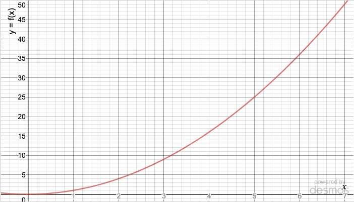Consider the function $f(x) = x^2,$ graphed to the right.

You know that at $x=3,$ $f(3) = 3^2 = 9.$

For now, we’ll simply tell you that the rate the function “climbs” at $x=3$ is exactly 6: \[\left.\dfrac{df}{dx}\right|_\text{at x = 3.00} = 6\] (Later we’ll show you how to determine this rate for yourself, a fundamental Calculus skill; Activity 2 below will also address this value. For now, so you can start doing “real” Calculus calculations, let’s just take the rate as a given.)

Use the information provided to find the (approximate) value of $f(3.01).$
Hint: The calculation is exactly the same as finding Syd’s vertical position $y(3.01).$
Although the approximation will be less good for reasons we’ll see, use the same approach to find the approximate value of $f(3.5).$

Solution.
(a) Let’s perform exactly the same calculation as we did to find Syd’s change in vertical position.
We know $f(3) = 9$ and $\left.\frac{df}{dx}\right|_\text{at x = 3.00} = 6,$ and we have $dx = 0.01.$
So using the same formulation as before:
\begin{align*}
\overbrace{f(x+dx)}^\text{$f$ value at $x+dx$} &= \overbrace{f(x)}^{\text{$f$ value at }x} + \overbrace{\text{ small change }df}^{\text{(rate at $x$)} * \, dx} \\[8px] f(3.01) = f(3 + 0.01)&= f(3) + (6) \cdot (0.01) \\[8px] &= 9 + 0.06 \\[8px] &= 9.06 \quad \cmark
\end{align*}
Note that the actual value is $f(3.01) = (3.01)^2 = 9.0601,$ so this is a pretty great estimate for such a quick calculation! We’ll discuss the tiny discrepancy between the values 9.06 and 9.0601 (a difference of 0.001%) below.

(b) The formulation for this calculation is the same, but now we have $dx=0.5:$
\begin{align*}
\overbrace{f(x+dx)}^\text{$f$ value at $x+dx$} &= \overbrace{f(x)}^{\text{$f$ value at }x} + \overbrace{\text{ small change }df}^{\text{(rate at $x$)} * \, dx} \\[8px]f(3.5) = f(3 + 0.5)&\approx f(3) + (6) \cdot (0.5) \\[8px] &\approx 9 + 3 \\[8px] &\approx 12 \quad \cmark
\end{align*}
The actual value is $f(3.5) = (3.5)^2 = 12.25,$ so this is a less-good estimate than we made in (a). We’ll discuss the larger discrepancy between the values 12 and 12.25 (a difference of 2%) immediately after this example.

Let’s now use the following Activities to dig in and see why in Example 1 the approximation for $(3.01)^2$ works well and yet doesn’t return the exact result, and why the approximation for $(3.5)^2$ works less well.

ACTIVITY 1.1: Zooming in on the curve $y=x^2$ around (3,9)

The interactive Desmos graph below shows the curve $y = x^2.$

Step 1. First, use the “+” button on the graph below to zoom in on the curve. Drag the curve as needed to keep the point $(3,9)$ near the center of the calculator’s window. (Text will appear on the graph as you zoom, and will tell you when to proceed to Step 2.)

Graph of $f(x) = x^2$ versus x

Step 2. You’ve just seen one of the key insights of Calculus: for most functions, when you “zoom in” sufficiently and look at a small region around a point of interest, the function’s curve looks like a line. And we like lines, a lot(!), because linear functions are super-easy to work with. Indeed, one MAJOR application of Calculus is to replace a small section of a function’s curve with an appropriate line segment. For instance, in the calculation you did to find $(3.01)^2$ above, we used the fact that the curve looks like a line with slope = 6 close to the point $(3,9).$

To see that this is so, first check this box to zoom the graph above to a convenient size:

Check/uncheck box to zoom the graph above.

And now compare that “curve” above with the line in the graph below: they are essentially indistinguishable – as long as we’re zoomed in sufficiently in the top graph.

Graph of line through $(3,9)$ with slope = 6

If you’d like, you can check this box to show the curve $y=x^2$ on this graph:

Check/uncheck box to show/hide the graph of $y=x^2.$

If you now zoom out and in, you can see how the green line and red curve look indistinguishable when you’re sufficiently zoomed-in, but are quite different when you’re zoomed-out.

The simple insight here about how the curve and line are indistinguishable when you’re sufficiently “zoomed in” in one of the key insights for all of Calculus.

LINEAR APPROXIMATION: Replace a bit of the curve with an appropriate line

As the preceding Activity illustrates, we can approximate a curve’s behavior by using the line instead, if we use an appropriate line, and if we stay within a region that is “close” to a particular point. Replacing a small section of a curve with a line of the correct slope in this way is known as a linear approximation. You can imagine that rather than walking along the curve itself, you’re instead walking along this short line that mimics the curve’s behavior. And we like lines, since they are much easier to work with than curves. The next activity shows how this handy replacement works mathematically.

ACTIVITY 1.2: Exploring the linear approximation

PART 1. Let’s tie the pieces together and revisit graphically the calculation we made in Example 1 above to find $(3.01)^2$. First, recall that calculation:
\begin{align*}
\overbrace{f(x+dx)}^\text{$f$ value at $x+dx$} &\approx \overbrace{f(x)}^{\text{$f$ value at }x} + \overbrace{\text{ small change }df}^{\text{(rate at $x$)} * \, dx} \\[8px] f(3.01) = f(3 + 0.01)&\approx f(3) + (6) \cdot (0.01) \\[8px] &\approx 9 + 0.06 \\[8px] &\approx 9.06
\end{align*}
The graph below once again shows $y = x^2,$ with the point $(3,9)$ highlighted.

Use the “+” button to zoom in, and drag the curve as needed to keep the point $(3,9)$ near the center of the window.
When you have zoomed in sufficiently, you’ll see a triangle appear with lines for dx and df. Zoom-in sufficiently so all of the numbers don’t overlap.
Use the slider beneath the graph to vary the value of dx.
Observe how for both positive and negative values of dx, the green line segment of the triangle very closely tracks the red line of the function’s curve.

Graph of $f(x) = x^2$ versus x

Use the slider to change the value of dx:

Currently dx = 0.010

Check/uncheck box to hide/show the $y=x^2$ curve.

You can use the checkbox above to hide/show the red curve $y=x^2.$ Check it now to hide the curve so you can focus on the triangle, which shows graphically the approximation-calculation you’re making.
We’ve repeated a smaller version of the same graph below, already zoomed-in. The same slider above controls the size of dx in it too. The calculation of the approximate value of $f(3+dx)$ is to its right, and if you change the value of dx you can see see how the calculation changes:

Graph of $f(x) = x^2$ versus x (repeated)

\begin{align*}
\overbrace{f(3+\color{blue}{dx})}^\text{$f$ value at $3+\color{blue}{dx}$} &\approx \overbrace{f(3)}^{\text{$f$ value at }3} + \overbrace{\color{green}\text{ small change }df}^{\text{(rate at $x=3$)} * \, (\color{blue}{dx})} \\[8px] f(3+\color{blue}{0.01}) &\approx 9+6(\color{blue}{0.01}) \\[8px] &=9+ \color{green}{0.06}\color{black}{=} \color{purple}{9.06}
\end{align*}

Fundamentally, you’re starting at the point we know exists on the curve $f(3)=9$, and then moving at the linear rate of $\left.\frac{df}{dx}\right|_\text{at x = 3.00} = 6,$ such that the small vertical change $df = 6 (dx).$
With this linear-approximation approach, you don’t actually need to know anything about the function other than (I) $f(3) = 9,$ and (II) $\left.\frac{df}{dx}\right|_\text{at x = 3.00} = 6.$ Indeed, it was with these two pieces of information that we we found Syd’s new position in Scenario 1 on the preceding screen, and $(3.01)^2$ and $(3.5)^2$ in Example 1 above.

PART 2. Let’s use some algebra to see why this linear approximation works. First, recall that
\[(a+b)^2 = a^2 + 2ab + b^2\] Since we have $f(x) = x^2,$ we can easily calculate the exact value of $f(3.01) = f(3 + 0.01)$:
\begin{align*}
f(3.01) = f(3+0.01) &= (3 + 0.01)^2 \\[8px] &= (3)^2 + 2(3)(0.01) + (0.01)^2 \\[8px] &= 9 + 6(0.01) + (0.01)^2 \\[8px] &= 9 + 0.06 + 0.0001
\end{align*}
You can now see how our linear approximation works: we keep the first two terms of the above expression, and ignore the third, squared (quadratic) term $(0.01)^2$, such that
\[f(3.01) \approx 9 + 0.06 = 9.06\] And we quickly see that the approximation is off by only the very small term $(0.01)^2 =0.0001$ that we dropped.

More generally, for any value of dx we have
\begin{align*}
f(3+dx) &= (3 + dx)^2 \\[8px] &= (3)^2 + 2(3)\, dx + (dx)^2 \\[8px] &= 9 + 6\,dx + (dx)^2
\end{align*}
Using our linear approximation approach, we again drop the quadratic $(dx)^2$ term, giving us an equation that depends linearly on dx:
\[f(3+dx) \approx 9 + 6\,dx\] We thus see why we’ve been using the rate near $x=3$ of $\left.\frac{df}{dx}\right|_\text{at x = 3.00} = 6:$ it’s the correct multiplicative factor for this linear approximation. We simply provided that value in Scenario 1 and Example 1 above; here we see through this algebraic approach where the value comes from. Note, however, that although in this case we could use simple algebra [expanding the quadratic $(3+dx)^2$] to find this rate, most functions do not allow for such an algebraic expansion. Hence a lot of our early work in the course will be to find ways to determine the rate of change for any function we encounter.

We’ve seen thus far that our linear approximation method works by replacing a function’s curve in a region around a specific point with a line that mimics the function’s behavior at nearby points. The approach of course introduces some error, since we’re following a line rather than the actual curve – and the farther we get from $x=3,$ the more the line deviates from the curve.

Let’s look more closely at this error that we introduce when using the linear approximation.

ACTIVITY 1.3: Explore the approximation error in dropping $(dx)^2$

We saw in Example 1 above that when we use the linear approximation method to calculate $(3+dx)^2,$ the percentage error when we calculate $(3.01)^2$ is only 0.001%. By contrast, the percentage error when we calculate $(3.5)^2$ is 2%, an error 2000-times as large.

PART 1: Approximation for $(3.5)^2$
Let’s look graphically at each calculation to see why the approximation gets worse as we move away from $x=3.$ We’ll look first at $(3.5)^2$. The exact value is
\begin{align*}
f(3.5) = f(3+0.5) &= (3+ 0.5)^2 \\[8px] &= (3)^2 + 2(3)(0.5) + (0.5)^2 \\[8px] &= 9 + 6(0.5) + (0.5)^2 \\[8px] &= 9 + 3 + 0.25 = 12.25
\end{align*}
On the graph below, we show this point on the red curve $f(x) = x^2$ as “Actual value: $f(3.5) = 12.25.$”

By contrast, our approximation throws away the $(0.5)^2$ term, so we have
\begin{align*}
f(3+0.5) &\approx 9 + 6(0.5) \\[8px]&\approx 9 + 3 = 12
\end{align*}
We show that point in the graph on the green line (with slope = 6) as “Approx value $f(3.5) \approx 12.$”

The vertical distance between those two points is exactly the approximation’s error, equal to $(0.5)^2 = 0.25.$
You might zoom out and in to get a sense for how the line is deviating from the curve here.

Approximating $(3.5)^2$

PART 2: Approximation for $(3.01)$
Let’s now look once again at our approximation for $(3.01)^2.$ The exact value is
\begin{align*}
f(3.01) = f(3+0.01) &= (3+ 0.01)^2 \\[8px] &= 9 + 6(0.01) + (0.01)^2 \\[8px] &= 9 + 0.06 + 0.0001 = 9.0601
\end{align*}
We show this point on the graph below as “Actual value: $f(3.01) = 9.0601.$”

By contrast, our approximation throws away the tiny $(0.01)^2$ term, so we have
\begin{align*}
f(3+0.01) &\approx 9 + 6(0.01) \\[8px] &\approx 9 + .06 = 9.06
\end{align*}
We show that point on the graph as “Approx value $f(3.01) \approx 9.06.$”

Approximating $(3.01)^2$

Notice that even though this graph is zoomed-in considerably more than the graph above, you still can’t even see the error initially. Instead you have to zoom in even further to see the gap of $(0.01)^2 = 0.0001$ between the approximate value and the actual value. The reason: the line is much closer to the curve for $dx = 0.01$ than for $dx = 0.5,$ which in turn is the reason we say dx needs to be “small.” Generally, the smaller dx is, the better our approximation will be.

Let’s consider another example function, one for which we’re dropping even more terms when we do our approximation.

Example 2: $g(x) = x^3$

Consider the function $g(x) = x^3,$ shown to the right.

You know that at $x = 1,$ $g(1) = (1)^3 = 1.$

We are given that at $x = 1,$ the function changes at the rate
\[\left.\dfrac{dg}{dx}\right|_\text{at x = 1} = 3\]

Using this information, find the approximate value of $(0.99)^3.$

Solution
We’ll use exactly the same approach as we did for Syd’s bike ride and as we did in Example 1. Note that this time dx is negative, $dx = -0.01,$ since the x-value we’re asked about (0.99) is a little less than the value we know about (at $x=1$).
\begin{align*}
\overbrace{g(x+dx)}^\text{$g$ value at $x+dx$} &= \overbrace{g(x)}^{\text{$g$ value at }x} + \overbrace{\text{ small change }dg}^{\text{(rate at $x$)} * \, dx} \\[8px] g(0.99) = g\big(1 + (-0.01)\big)&\approx g(1) + (3) \cdot (-0.01) \\[8px] &\approx 1 \,-\, 0.03 \\[8px] &\approx 0.97 \quad \cmark
\end{align*}
The actual value is $(0.99)^3 = 0.970299,$ a difference of 0.031%.
We’ll once again expore the error between our linear approximation and the actual value in the next Activity.

ACTIVITY 2.1: Exploring the error in the linear approximation for $(0.99)^3$

PART 1. Let’s tie examine graphically the calculation we made in Example 2 above to find the approximation to $(0.99)^3$.
The interactive Desmos graph below shows the curve $y = x^3,$ with the point $(1,1)$ highlighted.

Use the “+” button to zoom in, and drag the curve as needed to keep the point $(3,9)$ near the center of the window.
When you have zoomed in sufficiently, you’ll see a triangle appear with lines for dx and dg.
Use the slider beneath the graph to vary the value of dx.
Observe how for both positive and negative values of dx, the green line segment of the triangle closely tracks the red line of the function’s curve.

Graph of $g(x) = x^3$ versus x

Use the slider to change the value of dx:

Currently dx = -0.010

Check/uncheck box to hide/show the $y=x^3$ curve.

You can use the checkbox above to hide/show the red curve $y=x^3.$ Check it now to hide the curve so you can focus on the triangle, which shows graphically the approximation-calculation you’re making.
We’ve repeated a smaller version of the same graph below, already zoomed-in. The same slider above controls the size of dx in it too. The calculation of the approximate value of $g(3+dx)$ is to its right, and if you change the value of dx you can see see how the calculation changes:

Graph of $g(x) = x^3$ versus x (repeated)

\begin{align*}
\overbrace{g(1+\color{blue}{dx})}^\text{$g$ value at $1+\color{blue}{dx}$} &\approx \overbrace{g(1)}^{\text{$g$ value at }1} + \overbrace{\color{green}\text{ small change }dg}^{\text{(rate at $x=1$)} * \, (\color{blue}{dx})} \\[8px] g(1+\color{blue}{-0.01}) &\approx 1+3(\color{blue}{-0.01}) \\[8px] &= 1 – \color{green}{0.03}\color{black}{=} \color{purple}{0.97}
\end{align*}

PART 2. Let’s again use some algebra to see why this linear approximation works. First, recall that
\[(a+b)^3 = a^3 + 3a^2b + 3ab^2 + b^3\]

Don't remember $(a+b)^3$?

Most people don’t remember offhand the expansion of a cubic. But don’t let that throw you, especially on a test! Instead, start with what you know: the expansion of a quadratic, and go from there:
\begin{align*}
(a+b)^3 &= (a+b)(a+b)^2 \\[8px] &= (a+b)(a^2 + 2ab + b^2) \\[8px] &= (a^3 + 2a^2b +ab^2) + (ba^2 + 2ab^2 + b^3) \\[8px] &= a^3 + 3a^2b + 3ab^2 + b^3
\end{align*}

[collapse]

Since we have $g(x) = x^3,$ we can easily calculate the exact value of $g(0.99) = g\Big(1 + (-0.01) \Big)$:
\begin{align*}
g(0.99) = g\Big(1 + (-0.01) \Big) &= \Big(1 + (-0.01) \Big)^3 \\[8px] &= (1)^3 + 3(1)^2(-0.01) + 3(1)(-0.01)^2 + (-0.01)^3 \\[8px] &= 1\, -\, 3(0.01) + 3(0.0001) \,-\, 0.000001 \\[8px] &= 1\, -\, 0.03 + 0.0003\, -\, 0.000001 = 0.970299\\[8px] \end{align*}
You can now see how our linear approximation works: we keep the first two terms of the above expression, and drop the third term $3(-0.01)^2$ and the fourth term $(-0.01)^3)$, such that
\[g(0.99) \approx 1 \,-\, 0.03 = 0.97\] And we quickly see that the approximation is off by only the small terms that we dropped.

More generally, for any value of dx we have
\begin{align*}
g(1+dx) &= (1 + dx)^3 \\[8px] &= (1)^2 + 3(1)^2\, dx + 3(1)(dx)^2 + (dx)^3 \\[8px] &= 1 + 3\,dx + 3(dx)^2 + (dx)^3
\end{align*}
Using our linear approximation approach, we drop the third $3(dx)^2$ term and the fourth $(dx)^3$ term, giving us an equation that depends linearly on dx:
\[g(1+dx) \approx 1 + 3\,dx\] By the way, by expanding the polynomial we once again just developed the rate of change for the function $g(x) = x^3$ at $x=1$, $\left.\frac{dg}{dx}\right|_\text{at x = 1} = 3,$ which is the multiplicative factor for the linear approximation here. We can again do this because we had a simple polynomial we could expand in $(1+dx)^3.$ Remember that most functions do not allow for such an algebraic expansion, and so we still need to develop methods to determine the rate of change for any function we encounter.

The Examples and Activities above illustrate how linear approximations work: we keep only the linear term dx, which is known as the first-order term because it’s dx to the first-power. By contrast, we drop all of the higher-order terms, here the second-order term $(dx)^2$ and the third-order term $(dx)^3.$ We’ll learn much later in the course how to improve our approximations by including as many such higher-order terms as we’d like.

Time to practice some similar calculations for yourself! On the next screen you will find problems to practice with – each with a complete solution immediately available so you can easily check your work, or in case you need help. In the first problem you’ll see how you can use our linear approximation method to estimate $\sqrt{16.2}.$

Have a question or comment about the super-cool ideas on this screen? We’re getting to real Calculus now, based on the simple, everyday ideas you used on the preceding two screens. Please post your reactions and questions on our Forum!

The Upshot

For most functions $f(x),$ if we know the value of the function at a particular value of x, and its rate of change $\left.\dfrac{df}{dx}\right|_\text{at that value of x}$, then we can approximate the function’s value a small interval dx away:
\[f(x + dx) \approx f(x) + \overbrace{\text{ (rate at $x$)} * dx}^{df} \]
This “linear approximation” method replaces the curve in the region close to the point we know about with a line segment that changes at the same rate as the original function at that point.
The linear approximation is a first-order approximation, since we keep the linear term dx but discard all higher-order terms (those involving $(dx)^2,$ $(dx)^3,$ and so forth).
The smaller the size of dx, the better the approximation is likely to be.

Don’t wait: Start getting these ideas into your head, and hands, now by doing a related problem or two. It’s all free, and of course the only way to learn something is by doing it for yourself!

We'd appreciate your feedback! 😊

How helpful?

That's great to hear, thanks! If you have any requests or suggestions for us, we'd love to hear them. (If not, please just hit 'Submit.')

Thanks for your input. If you'd like to tell us, what would have made the material more helpful for you? (If not, please just hit 'Submit.')

Thanks very much for your input. Our aim is to help you do well! If you'd like, please tell us what would have been more useful, and we'll use that to improve. (If not, please just hit 'Submit.')

We're sorry you didn't find this helpful and appreciate your letting us know. Our aim is to help you do well! If you'd like, please tell us what would have been more useful, and we'll use that to improve. (If not, please just hit 'Submit.')