To conclude our study of limits and continuity, let’s introduce the important, if seemingly-obvious, Intermediate Value Theorem, and consider some typical problems. We’ll need the theorem later for some of our more important Calculus-y proofs, but even on this screen we’ll see some surprising implications. (At the bottom of this screen, we’ll look — optionally — at how Desmos graphs are often misleading essentially because of misuse of this theorem. No knock on Desmos, which we love and use a lot as you’ve seen! Even they say you must be aware of its limitations, including the ones we’ll see below.)
To understand the theorem, take a look at the top figure: the function f is continuous on the interval $[-3, 5].$ As you can see, its curve starts at the point $(3, -4)$ and ends on the point $(6, 5).$ No surprise: between $x=3$ and $x=5$ the function takes on all output values between $y=-4$ and $y=5.$
By contrast, the lower figure shows the function g which is not continuous on the same interval $[-3, 5]$; instead, it has a gap. And because it’s not continuous on the interval, we cannot be sure that it takes on all of the same output y-values that f does. (Seems obvious, right?)
IVT = Intermediate Value Theorem
The simple contrast between the functions f and g here illustrates an extremely important consequence of a function being continuous, and that consequence is captured by the Intermediate Value theorem (which we’ll frequently abbreviate as “IVT”):
Intermediate Value Theorem (IVT)
If a function f is continuous on a closed interval $[a, b]$ and if $f(a) \ne f(b),$ then f takes on every value between $f(a)$ and $f(b)$ in the interval $[a, b].$
A common use of the IVT is to prove that an equation has at least one solution, even if you don’t immediately (or ever) know what that solution is. The next example illustrates.
Example 1: Solution existence
Show that the equation $-2x^3 +5x^2 -4x + 10 = 8$ has a solution in the interval $[1, 2].$ (Of course: don’t use a calculator or other device to simply find the solution.)
Solution. Notice that the question doesn’t ask us to find the solution; instead, it asks us to show that a solution exists. This is a strong clue that we should use the IVT.
First, let $f(x) = -2x^3 +5x^2 -4x + 10.$ Since f is a polynomial, and as we saw on the preceding screen polynomials are continuous everywhere, f is continuous everywhere. (This is important to state in order to invoke the IVT!)
Next, let’s compute the value of f at the endpoints of the interval $[1, 2]$: \begin{align*} f(1) &= -2(1)^3 + 5(1)^2 -4(1) + 10 = 9 \\[8px]
f(2) &= -2(2)^3 + 5(2)^2 -4(2) + 10 = 6 \end{align*} Perfect: the question asks us to show that a solution exists for $f(x) = 8,$ and since 8 lies between 9 and 6 we can invoke the IVT:
Since f is continuous and $f(1) = 9$ and $f(2) = 6,$ by the IVT we know there is at least one input-value c where $1 \le c \le 2$ such that $f(c) = 8. \quad \cmark$
We note the following corollary to the IVT which is often easier to use in practice:
Corollary to the Intermediate Value Theorem, useful for existence of a root
If f is continuous on $[a, b]$ and $f(a)$ and $f(b)$ have opposite signs, then there is a number c between a and b such that $f(c) = 0.$
The corollary is useful because if you yourself have to supply the values of a and b, initially by just guessing, then it’s easier to try and hone in on values with the goal of finding just one output-value that’s negative and one that’s positive. You then know that the curve must cross the x-axis somewhere between your two input values. The following example illustrates, and also introduces one super-helpful problem-solving tip.
Example 2: Solution exists for $2 -x = 2^x$
Show that there is at least one solution to the equation $2 -x = 2^x.$
Solution. Notice again that the question doesn’t ask us to solve the equation, but rather to show that a solution to $2 -x = 2^x$ exists. We thus again turn to the IVT.
A VERY HELPFUL initial move is to rewrite the given equation and introduce a new function \[f(x) = (2-x) -2^x\]
because now we have the simpler task of showing that there is some number c such that $f(c) = 0.$ Note, crucially, that f is continuous for all x since it is comprised of a polynomial and an exponential function, so we can apply the IVT to it.
We now just start guessing at values of a and b with the goal of finding outputs with opposite signs, since that guarantees that there is a value of c between a and b such that $f(c) = 0$ as we desire.
So let’s start guessing. The easiest number to try is 0: \[f(0) = 2 -0 – 2^2 = 1 \implies \text{a POSITIVE value} \]
Great: we have our positive value. Now let’s search around for a negative value, first trying $x=-1$: \[f(1) = 2 – (-1) -2^{-1} = 3 – \dfrac{1}{2} \implies \text{a more-positive value} \] Oops: that didn’t help, since we got another positive output. No matter: let’s try another value, going to the positive-side of $x=0$. . .
and let’s try $x=1$: \[f(1) = 2 – 1 -2^1 = -1 \implies \text{a NEGATIVE value}\]
Perfect! We now have \[f(0) = 1 \gt 0 \quad \text{and}\quad f(1) = -1 \lt 0\]
and so by the IVT we know that there is a value of c between $x=0$ and $x=1$ such that $f(c) = 0.$ That in turn means that c satisfies $4 – c = 2^c,$ as requested. $\; \cmark$
Furthermore, not that the question asked, but we know that the value of c lies in the interval $(0 , 1).$
Example 2 illustrates the helpful move of defining a new function f (or g or whatever) at the start of a solution so you’re looking for a value of c such that $f(c) = 0.$ It might initially feel weird to define a new function for yourself to work with, but really you’re just rewriting the expression you were initially given and putting it into a form where you can set $f(x) = 0.$
The following example is another illustration of this helpful tactic — and also an example of how we can apply the IVT to some surprising scenarios.
Example 3: Height and weight with equal values?
True or False? At some time t since you were born, your weight in pounds equaled your height in inches.
Solution. This question seems out-of-the-blue . . . but we note that this question again doesn’t ask for the value of the time t, and instead just asks about whether such a moment exists. And that again is a clue to use the IVT.
One way to show that this statement is true is to, following the Problem-Solving Tip, define a new function that is the difference between the two quantities of interest. So let’s define a function that’s the difference between your weight as a function of time, and your height as a function of time: \[f(t) = \text{ weight}(t) – \text{ height}(t)\]
Since both weight and height are continuous functions of time, f is continuous.
Now, note that at birth, $f(\text{birth}) \lt 0$ whereas $f(\text{today}) \gt 0.$
Hence by the Intermediate Value Theorem, there must be some particular moment T between your birth and now when $f(T) = 0$, and hence when your weight (in pounds) was equal to your height (in inches). The statement is thus true. $\; \cmark$
Note that we don’t know when that moment was, only that it must exist.
Here are some practice problems for you to try.
Practice Problems
Practice Problem #1
True or False? You were once exactly 2 feet tall.
Show/Hide Solution
True. You were less than 2 feet tall when you were born, and today you are (we assume) taller than 2 feet. Since your growth is continuous, according to the Intermediate Value Theorem there must be a moment between when you were born and today when you were exactly 2 feet tall. Note that we don’t know exactly when that moment was; only that it must exist.
If you’d like to track your learning on our site (for your own use only!), simply log in for free
with a Google, Facebook, or Apple account, or with your dedicated Matheno account. [Don’t have a dedicated Matheno account but would like one? Create your free account in 60 seconds.] Learn more about the benefits of logging in.
It’s all free: our only aim is to support your learning via our community-supported and ad-free site.
[hide solution]
Practice Problem #2
Show that the function $f(x) = -3x^3 - 2x^2 +3x +1$ has a zero between $x = -1$ and $x =0$. Note: You may not use a calculator to answer this question.
Show/Hide Solution
Since $f(x)$ is a polynomial, it is continuous. We can therefore use the Intermediate Value Theorem (IVT). We’ll compute $f(-1)$ and $f(0)$, and hope that one turns out negative and the other turns out positive, because then we know by the IVT that there must be a number $c$, $-1 So let’s compute those two values:
\begin{align*}
f(-1) &= -3(-1) – 2(1) + 3(-1) +1 = -1\\
f(0) &= -3(0) – 2(0) + 3(0) +1 = 1
\end{align*}
Ah, as we were hoping. Since $f(-1)
If you’d like to track your learning on our site (for your own use only!), simply log in for free
with a Google, Facebook, or Apple account, or with your dedicated Matheno account. [Don’t have a dedicated Matheno account but would like one? Create your free account in 60 seconds.] Learn more about the benefits of logging in.
It’s all free: our only aim is to support your learning via our community-supported and ad-free site.
[hide solution]
The next problem is often found in textbooks, and sometimes on exams.
Practice Problem #3
Is there a number that is exactly 1 more than its cube? Note: You may not use a calculator to answer this question.
Show/Hide Solution
Many students have no idea what to do when faced with this brief question. Here’s how to approach it.
First, note that the question is not asking you to find this number; instead, it is asking whether such a
number exists. And that is a BIG CLUE we should think about the Intermediate Value Theorem (IVT). With that in mind, we start by expressing the statement mathematically:
Is there some number, $x$, that is exactly 1 more than its cube, $x^3$. That is, is there a solution to the equation
\[x = x^3 + 1 \text{ ?}\] As we noted above, when asked whether two expressions are ever equal, it’s helpful to define a new function that is the difference between those two expressions. Hence we define $f$:
\begin{align*}
f(x) &= x^3 + 1 – x \\ \\
&= x^3 -x +1
\end{align*}
The question now becomes whether there exists a solution to $f(x) = 0$.
Note that since $f(x)$ is a polynomial, it is continuous. Hence we can use the IVT to prove that
there exists a solution to $f(x) = 0$. . . if we can find some number $a$ such that $f(a) \gt 0$, and some number
$b$ such that $f(b) \lt 0.$ Then, by the IVT we know that there is a value
$c$ between $a$ and $b$ for which $f(c) = 0$, and we’re done!
So now, we just try out some numbers and see what happens. The easiest number to try is 0:
\[f(0) = 1 \text{, which is } > 0\]
So we already have a value for $a$ such that $f(a) > 0$.
Now let’s look for $b$ such that $f(b) \lt 0$. The next-easiest number to try is 1:
\[f(1) = 1 -1 + 1 = 1 \text{, which is also } > 0\]
and so doesn’t work. Let’s next try $-1$:
\[f(-1) = -1+1 + 1 = 1 \text{, which is again } > 0\]
and so again doesn’t advance us.
Having exhausted those really-easy numbers to try, let’s stop and think a bit: we want $f(x)$ to be negative, and we know we substitute larger values, $x^3$ will dominate over $x$. Hence we’ll try only negative numbers from now on. Let’s try the next-easiest negative number, $-2$:
\[f(-2) = -8 + 2 + 1 = -5 \text{ which is } \lt 0\]
So that works as $b$ such that $f(b) \lt 0$! We’re essentially done, but should wrap things up by summarizing:
“For the function $f(x)$ defined above, $f(0) > 0$ and $f(-2) \lt 0$, and so by the IVT there exists a number $c$, $-2 \lt c \lt 0$, such that $f(c)=0$. Hence there exists a number $c$ that is exactly 1 more than its cube.” $\quad \cmark$
Furthermore, although the question doesn’t ask us to go any further, we actually have shown that the value of x we’re after lies in the range $[-2, -1].$
If you’d like to track your learning on our site (for your own use only!), simply log in for free
with a Google, Facebook, or Apple account, or with your dedicated Matheno account. [Don’t have a dedicated Matheno account but would like one? Create your free account in 60 seconds.] Learn more about the benefits of logging in.
It’s all free: our only aim is to support your learning via our community-supported and ad-free site.
[hide solution]
Practice Problem #4
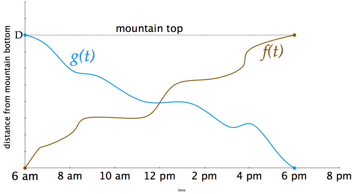
A hiker starts walking from the bottom of a mountain at 6:00 a.m., following a path, and arrives at the top of the mountain at 6:00 p.m. The next day she starts from the top at 6:00 a.m. and takes the same path to the bottom of the mountain, arriving at 6:00 p.m. Prove using the intermediate value theorem that there is a point on the path that the hiker will cross at exactly the same time of the day on both days.
Show/Hide Solution
Before we use the theorem to prove the statement, let’s imagine a slightly different situation to develop an intuitive understanding of what’s going on. Picture a hiker, Fran, who starts at the bottom of the mountain at 6:00 a.m and hikes up along the only existing path toward the top. Also imagine a second hiker, Greg, who starts his hike simultaneously with Fran at 6:00 a.m.—but Greg starts his hike from the top of the mountain, and heads down along the same single path. Fran finishes her hike at 6:00 p.m., arriving at the top of the mountain; Greg also finishes his hike at 6:00 p.m., arriving at the bottom of the mountain at that same moment. Now clearly Fran and Greg must pass each other at some point during the hike, since they’re on the same path and both hike for exactly the same 12 hours. We don’t know when their paths cross; indeed, the exact moment depends on how fast each hikes, when they take their breaks, and other details of their separate walks. But regardless of those details, we know that there is some moment when they cross paths. The argument remains the same if we replace Greg’s hike with Fran’s return trip the following day: since she starts at 6:00 a.m. and finishes at 6:00 p.m., and follows the same path, there must be some moment when she is at the same location she was the day before at that time. (If it’s easier to picture, imagine the downward-headed Fran meeting her upward-headed twin who left the bottom of the mountain at 6:00 a.m. Their paths must cross at some point, even if we don’t know exactly when.) To make our argument more formal, let the function $f(t)$ represent Fran’s distance along the path, as measured from the bottom of the mountain, on the first day or her hike. Hence $f$(6:00 a.m.) = 0, since she starts at the bottom of the mountain. Let’s say that when she reaches the top of the mountain, she has traveled a distance $D$ along the path, such that $f$(6:00 p.m.) = $D$. (See the graph: one possibility for $f(t)$ is shown in brown.) Note that $f(t)$ is a continuous function, since Fran moves continuously along the path: she can’t suddenly disappear from one spot and suddenly appear in another without traversing the points in-between. Now let the function $g(t)$ represent Fran’s distance along the path, as measured from the bottom of the mountain, on the second day of her hike, when she takes her return trip. (We first imagined this above as Greg’s hike down the mountain.) Since she starts this hike at 6:00 a.m. at the top of the mountain, $g$(6:00 a.m.) = $D$. At the end of her hike, we have $g$(6:00 p.m.) = 0. (One possibility for this function is shown on the graph in blue.) Note that $g(t)$ is also a continuous function, for the same reason $f(t)$ is. As you can see in the graphic, no matter the exact shape of two curves representing the two functions, they must cross at some point. We can’t say exactly where they cross without more information, but we know they must cross somewhere. To use the Intermediate Value Theorem, let’s invoke an approach we’ve now used several times above, and create a new function, $h(t)$, that is the difference of the two functions above: $$h(t) = g(t) – f(t)$$ Now, at the start of the day, $h(\text{6:00 a.m.}) = g(\text{6:00 a.m.}) – f(\text{6:00 a.m.})= D – 0 = D.$ By contrast, at the end of the day $h(\text{6:00 p.m.}) = g(\text{6:00 p.m.}) – f(\text{6:00 p.m.})= 0 – D = -D.$ Since $0$ is between $D$ and $-D$, by the Intermediate Value Theorem there must be a time $T$ between 6:00 a.m. and 6:00 p.m. such that $h(T) = 0$. That is, there must be some instant when the two functions have the same value—which means that she is at the same spot on the path at exactly the same time of the day on both days. Again, we would need more information to know when that time of day is, but regardless, we know that it must exist. $\quad \cmark$
If you’d like to track your learning on our site (for your own use only!), simply log in for free
with a Google, Facebook, or Apple account, or with your dedicated Matheno account. [Don’t have a dedicated Matheno account but would like one? Create your free account in 60 seconds.] Learn more about the benefits of logging in.
It’s all free: our only aim is to support your learning via our community-supported and ad-free site.
[hide solution]
This next problem is a little mind-blowing, at least to us, but follows the same type of reasoning as the preceding questions.
Practice Problem #5
Two points on the surface of the Earth are called antipodal if they are at exactly opposite points. (For example, the North Pole and South Pole are antipodal points). Prove that, at any given moment, there are two antipodal points on the equator with exactly the same temperature. Hint: Let $T(\theta)$ be the temperature, at any given moment, at the point on the equator with longitudinal angle $\theta$ measured in radians, $0 \le \theta \le 2\pi$. (That is, in one complete trip around the equator, $\theta$ goes from 0 to $2\pi$.) Consider the function $f(\theta) = T(\theta + \pi) - T(\theta)$.
Show/Hide Solution
We don’t find the result that the question is asking to prove to be intuitive at all; in fact we find it remarkable. It is nonetheless true. Before we follow the hint and launch into the proof, we can develop some understanding by considering two points on the opposite sides of equator, using the function that the hint defines: $$f(\theta) = T(\theta + \pi) – T(\theta)$$
For simplicity, let’s first consider the point with longitude $\theta_a = 0$ radians (in the Atlantic Ocean); then its antipodal point has longitude $\theta_a + \pi = \pi$ radians (in the Pacific Ocean). Furthermore, let’s suppose for the moment that $T(0) > T(\pi)$. With that assumption, the difference between the two functions is negative:
$$f(0) = T(\pi) – T(0) T(\pi)$; it won’t matter for the argument, so let’s just suppose that it is.) Now imagine increasing $\theta$, bit by bit, sweeping around the Earth’s circumference. Since the temperature varies continuously as we move around the circle, $f(\theta)$ varies continuously too. We keep sweeping around until we come to the opposite side of the Earth, where $\theta_b = \pi$. But note that we’re comparing the same two points as we did before—the points with longitude $\pi$ radians (in the Pacific) and $2\pi$ radians (which is the same as 0 radians, back where we started in the Atlantic). But their order has reversed when we compute $f(\theta)$: \begin{align*}
f(\pi) &= T(2\pi) – T(\pi) &&\text{[Note that $T(2\pi) = T(0)$]}\\ \\
&= T(0) – T(\pi) \\ \\
&= -f(0) \\ \\
&> 0
\end{align*}
So we started with $f 0$, and hence (since $f$ is continuous) by the Intermediate Value Theorem there must be a point somewhere between 0 and $\pi$ radians along the equator such that $f = 0$, i.e., where that point and its antipodal point have the same temperature. If you were to encounter this or a similar question on an exam, we suggest just jumping in with the hint and seeing where it takes you. (Don’t just stare at the blank page; start by writing down something that the problem told you!) The hint was
$$f(\theta) = T(\theta + \pi) – T(\theta)$$
Since temperature is a continuous function on the Earth’s surface, $f(\theta)$ is a continuous function. With no further guidance provided by the hint, let’s write an expression for $f$ at some particular angle alpha: $\theta = \alpha$.
$$f(\alpha) = T(\alpha + \pi) – T(\alpha) \; \blacktriangleleft $$
Since that expression contains $T(\alpha + \pi)$, let’s also write the expression for $f(\alpha + \pi)$ just to see what happens:
$$f(\alpha + \pi) = T(\alpha + 2\pi) – T(\alpha + \pi)$$
But note that $T(\alpha + 2\pi) = T(\alpha)$ since $T$ is a periodic function with period $2\pi$. (That is, we’ve just swept all the way around the circle to back where we started.) Hence we can rewrite the preceding line: $$f(\alpha + \pi) = T(\alpha) – T(\alpha + \pi)$$
Comparing that to our expression for $f(\alpha)$ above $(\blacktriangleleft)$, we see that
$$f(\alpha + \pi) = -f(\alpha)$$
Let’s consider the possibilities here:
If both $f(\alpha + \pi)$ and $f(\alpha)$ are zero, then that particular value of $\alpha$ specifies a point that has the same temperature as its antipodal point at $\alpha + \pi$, and we’ve shown what we were after. If they are not zero and $f(\alpha)$ is positive, then the last expression tells us that $f(\alpha + \pi)$ is negative; if $f(\alpha)$ is negative, then $f(\alpha + \pi)$ is positive. Hence by the Intermediate Value Theorem, there must exist an angle we’ll call $\theta_c$ in $(0, \pi)$ for which $f(\theta_c) = 0$, and hence where the point specified by $\theta_c$ and its antipodal point at $\theta_c + \pi$ have the same temperature. $\quad \cmark$ As an aside, this remarkable fact about two anitpodal points having the same temperature is a specific application of something called the Borsuk–Ulam Theorem.
If you’d like to track your learning on our site (for your own use only!), simply log in for free
with a Google, Facebook, or Apple account, or with your dedicated Matheno account. [Don’t have a dedicated Matheno account but would like one? Create your free account in 60 seconds.] Learn more about the benefits of logging in.
It’s all free: our only aim is to support your learning via our community-supported and ad-free site.
[hide solution]
We promised at the top of the screen a discussion of a way in which Desmos and other graphing programs are sometimes entirely misleading. Open the box if you’re interested:
Optional look at one way Desmos and other graphing programs are sometimes wrong(!)
The interactive graph below shows a function we’ve looked at often: $f(x) = \dfrac{x^2 -4}{x-2}.$ What do you notice about what the graph shows for the value of $f(2)$?
Misleading graph of $f(x) = \dfrac{x^2-4}{x-2}$
You of course know that $f(2)$ is undefined, since the function’s denominator equals zero when $x=2.$ But no matter how much you zoom in, the red line passes straight through the point $(2,4)$ — which is quite misleading! (To Desmos’s credit, if you slide your cursor along the line, when you reach $x=2$ Desmos shows the point as “(2, undefined),” which is correct. It’s just the graph’s continuous red line itself that is misleading.)
We’re not showing you this to criticize Desmos; we love them! (As you can tell by the amount we use them throughout our materials here. This site would be much different, and worse, without them.) And FYI, almost every graphing calculator and app functions makes this same “mistake.”
Rather, we strongly believe that it’s important to understand the limitations of any tool that you use, which in turn means developing an understanding of how the tool works. In this case, that tool is Desmos’s graphing engine. And really, that engine — while truly amazing — isn’t very smart.
Instead, it uses brute force: when you enter an expression, the calculator gets to work and quickly calculates a large number of points, plots them, and then essentially connects the dots so you see a smooth curve — thereby assuming the function is continuous. That is, it implicitly uses the IVT and “fills in” all of the values between the ones it has calculated. Of course a consequence of this approach is that when the function is not continuous, as this one isn’t at $x=4,$ you simply get a misleading graph.
For this reason, behind-the-scenes in every graph you’ve seen up to this point we’ve manually added the open-circle for the point $(2,4)$ to make the graph correct. To see this for yourself, tap the “>>” in the upper left of the graph to reveal the expressions list. If you then tap the circle in the expression for the point $(2, 4),$ you’ll see the open-circle that we always put in place.
Again, the point of this discussion is not to criticize Desmos or any other graphing tool. Instead, we want to emphasize the importance of building your own mathematical knowledge so you can recognize when a graph is showing you something that isn’t quite right . . . and now, we hope, also understand why that’s happening.
[collapse]
What questions or comments about the IVT, or continuity, or limits do you have? Please pop over to the Forum and join the discussion with the rest of the community, including us!
The Upshot
The Intermediate Value Theorem (IVT) states the obvious fact that: If a function f is continuous on a closed interval $[a, b]$ and if $f(a) \ne f(b),$ then f takes on every value between $f(a)$ and $f(b)$ in the interval $[a, b].$
Its corollary is often more useful in practice: If f is continuous on $[a, b]$ and $f(a)$ and $f(b)$ have opposite signs, then there is a number c between a and b such that $f(c) = 0.$
A very strong clue to use the IVT (or more likely, its corollary) is that a problem statement asks you to “show that a solution exists,” or that the function takes on a particular output-value somewhere between two input-values; the problem does not ask you to find the solution, or the specific input-value where the output-value occurs. For such problems, use the steps outlined in the Examples and Practice Problems above.
Chapter Conclusion, and What’s Next
And with that, we conclude our study of limits and continuity.
A function’s average rate of change over an interval is equal to the slope of the secant line that passes through the endpoints of the interval: \[\text{average rate of change}_{[x_1,\, x_2]} = \text{slope of line segment} = \frac{\color{purple}{\Delta y}}{\color{green}{\Delta x}} = \frac{\color{purple}{f(x_2)- f(x_1)}}{\color{green}{x_2\, -\, x_1}}\]
You can make the average rate of change arbitrarily close to the instantaneous rate of change at $x_1$ by making $x_2$ sufficiently close to $x_1$ (and hence $\Delta x$ sufficiently small).
These points raise a natural question that led to the development of Calculus itself:
How small can we make $\Delta x$??
We know it can’t be exactly zero, because we can’t divide by zero in the slope calculation. So how small can we make it?
We will take up this key question – arguably THE key question – when we explore THE key tool in Calculus in the next Chapter, on “Limits”.
We now have that we have that foundational tool of limits — without which Calculus wouldn’t exist! — and so we can return to that question. The answer will lead us to develop one of the (only) two fundamental concepts of Calculus, the derivative, in the next Chapter. . . which we will have available soon. We will be excited to see you there when it’s ready — please watch the Forum for the announcement when it’s available.
For the moment, we hope you’ll have a small celebration for yourself: understanding the concept of “the limit” deeply means understanding one of the great triumphs of science and mathematics. (There’s a reason the founders of Calculus are so celebrated!) We sincerely hope we’ve helped you lay a firm foundation for yourself from which to build the key ideas to come. If you would be so kind, please let us know on the Forum: we really need and appreciate your feedback.
And please don’t forget that celebration part!
If we've helped you learn something, perhaps you'd like to give back a little something and
☕ Buy us a coffeeWe're working to add more, and would appreciate your help to keep going! 😊
Once you log in with your free account, the site will record and then be able to recall for you:
Your answers to multiple choice questions;
Your self-chosen confidence rating for each problem, so you know which to return to before an exam (super useful!);
Your progress, and specifically which topics you have marked as complete for yourself.
Your selections are for your use only, and we do not share your specific data with anyone else. We do use aggregated data to help us see, for instance, where many students are having difficulty, so we know where to focus our efforts.
You will also be able to post any Calculus questions that you have on our Forum, and we'll do our best to answer them!
We believe that free, high-quality educational materials should be available to everyone working to learn well. There is no cost to you for having an account, other than our gentle request that you contribute what you can, if possible, to help us maintain and grow this site.
Please join our community of learners. We'd love to help you learn as well as you can!
We use cookies to provide you the best possible experience on our website. By continuing, you agree to their use.OK

![Graph showing the point (1,9) and text: We know for the interval [1, 2] the curve starts here. Then the point (2, 6) with the text: and ends here. More text: Since f is continuous, we thus know by the Intermediate Value Theorem that the curve _must_ include a point with y=8. (We don't know where exactly, but we know the point exists](https://sp-ao.shortpixel.ai/client/to_webp,q_glossy,ret_img,w_757,h_447/https://www.matheno.com/wp-content/uploads/INT-Ex1.png)


What are your thoughts or questions?